Modeled Elevation POI Change with Variables: MV and Air Temperature

[Biologist]

Part 1:

Introduction:

I am interested in how the outside air temperature (and therefore its density and air resistance properties), variability affects bullet speed and drop (vertical POI), across a range of muzzle velocities.

I shoot benchrest rimfire at 50m all winter at my local range where we are fortunate to have a heated shooting house, from which we shoot outdoors through window ports for each bench. Over a year we might shoot a range of temperatures between about -35C to +30C. Therefore, the air resistance properties should, in theory, be significant for POI shifts on target across these wide temperature ranges.

Methods:

To investigate this, I used JBM Ballistics program (free online version) to run some theoretical scenarios with 2 independent variables of MV and air temperature.

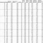
To calculate the absolute drop, I recorded JBM's output for "time of flight" to 50m for each MV and air temperature scenario combination. Time of flight squared, multiplied by the Gravitational Constant (9.8m/s/s), provides the absolute drop over 50m.

Note: There are no barrel harmonics variables in this model. We are simply isolating air temperature and MV in the model for investigation.

Inputs for the JBM Ballistics scenarios: (note: all of these are held constant, so they should not matter for comparing the differences or delta absolute drop’s):

Cartridge and Bullet: 40 gr, chosen from JBM's library list: It looks to be an old list, and I could not find the current Lapua, Eley and SK lines of ammo I use. So, I just picked one that looked close: Lapua "Midas M". I don't know this line of ammo. But it should not matter anyways, since the bullet's inputs (BC, length) are held constant.

Pressure: Set to 985 mb. (average for my home range).
Altitude: 1000 ft.
Relative humidity: 50%
Twist: 1:16

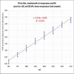
If this works, I was hoping that I could generate a linear graph of variance, fit a regression line to it with Excel, and then I would have an equation that we could compare to observed real data using a chronograph and weather meter.

Part 2 next shows the modeled results with data and graphs.

 

[Biologist]

Part 2:

Methods (continued):

The data chart is below. I used a temperature range of -20C to +30C, to capture the range most folks will be shooting in. I used a MV range of 950 fps to 1125 fps to represent the commonly used subsonic target ammo.

The output value from JBM Ballistics is the "time to target". That value is then squared to get seconds squared. That value is then multiplied by 9.8m/s/s. That product returns the absolute drop in meters. That drop in m is converted to inches and mm.

Results:
The maximum absolute drop was, not surprisingly, the coldest temperature (-20 C) and slowest MV (950 fps) at -12.50 inches absolute drop. I used this as the zero elevation. Adding 12.50 to each negative drop distance produced the positive POI elevation gain (inches up) from the zero'd value.



The graph below is the POI at 50m modeled with the various at temperatures and MV's. Some of the plots overwrite each other because the values are identical or very close at this scale.



Note there is a very slight curve downwards of the lines from slower to faster MV's, i.e. a slower rate of increase of elevation gain for POI. This curve is expected because the relationship is not purely linear. Air resistance increases by the square as velocity increases for a given temperature.

As air temperature increases, air density decreases and therefore air resistance decreases for a given velocity, so the trend is still upwards as velocity increases, but at a dampening angle. Its up to the Ballistics calculator to account for these variables, so what you see is what JBM is doing. Its not necessarily accurate because all models are wrong and simplified. The model's practical value is more in the general trend output.

Conclusions:
According to JMB’s modeled calculations, we would expect:

1) A POI difference of about 3.5 inches at 50m across the full range of air temperature and MV's.
2) For any given MV, we would expect about 0.3 to 0.5 inches POI shift across the air temperature range of -20C to +30C. For an MOA scope elevation turret, at 50m that is roughly a 3/4 to 1 MOA range of adjustment clicks to cover this 50 degrees C of air temperature change. From 0C to 30C we would expect about 0.25 inches, or about 1/2 MOA adjustment.

In Part 3 we look at the slope of the trend and the regression line and see how to predict POI differences for any MV and air temperature.

 

[Biologist]

Part 3:

Results (continued):

The graph below is the same values, pooled together to see if we can derive a trend line.

Excel provides a regression function, and it generated the trend line of best fit to the POI variance data. The red line is the regression trend line, and its equation and R squared value.



The equation of the trend line is Y = 0.018X – 16.803.

The R squared value is 0.9754.

Conclusion:

The R squared is very high at 0.9754, indicating that about 97.5% of the variance in the POI data can be explained by the regression of MV and air temperature.

Caution: The relationships are subject to all the assumptions built into the JBM Ballistics models, and specifically its accuracy for calculating the bullet’s flight time to target. Other models will likely produce different absolute values in the tables.

Part 4 next, is the Discussion....

 

[Biologist]

Part 4:

Discussion:

OK, after all this, so what? Is this even useful?

Its there to play around with to see if your MV's variance produces similar or different delta POI shifts for elevation.

If you know your ammo lot's MV ES, it can maybe give you a ballpark estimate of what to expect for POI variance at 50m in a score match, or shooting for group. E.g., If your ammo lot's ES is 50 fps for your fired rounds, at 50m don't expect to shoot half inch groups, or don't expect to score a perfect 10-X for every score shot. With an ES of 50 fps, you would be closer to shooting 3/4 inch elevation variance, according to this model.

NOTE: Obviously in the abstract modeling world, the bullets are all perfectly identical and all fly exactly as the model dictates. We know in the real world that all bullets are not the same. There are dents on the heel and bottom, and there are concentricity irregularities or center of gravity variances, bullet to bullet, that make them fly not perfect, and therefore they all do not obey the model's trajectory based on MV. This simple model does not account for barrel "bang" harmonics for different MV's. This equation and trend line will not account for these issues.

What the model outputs may be useful for, is understanding the magnitude of POI elevation shifts within your lot of ammo, if you know your lot's MV ES.

I am interested in your comments, and any real world data you can plug into that equation to see if your delta POI comes close to the model's predictions.

EDIT: See Post #9 for examples for how to plug in MV's to the equation and predict POI elevation shifts.

 

[horseman2]

You would obviously sight in every time you go to the range so you are creating a constant.

Shooting from a heated shooting house creates a variable that would not appear to be calculated in to the program.
How warm can the temperature be set in the shooting house?

I wear a shirt on cold days and keep my ammo in a pocket close to my heart. I also have some handwarmers tht will keep the temperature up in the ammo bucket.

 

[grauhanen]

This obviously represents a good amount of time and effort and that's appreciated. I will have to give it some time and effort myself to more fully understand the information and its implications.

 

[Biologist]

You would obviously sight in every time you go to the range so you are creating a constant.

Shooting from a heated shooting house creates a variable that would not appear to be calculated in to the program.
How warm can the temperature be set in the shooting house?

I wear a shirt on cold days and keep my ammo in a pocket close to my heart. I also have some handwarmers tht will keep the temperature up in the ammo bucket.

Yes. Sighting in controls your POI, when you figure that out with sighters. Sighting in is the correction for absolute drop on any given day. Absolute drop is pure gravitational force perpendicular to the center of the earth that is a constant (9.8 m/s/s), as a function of flight time to target. That is why 100% of the delta of the absolute drop can be accounted for by time to target. The absolute drop accelerating force vector (gravitational force constant) is the same regardless of whatever angle your bore axis is to the target.

What about spindrift, which creates an additional force downwards to the right ? (and there was no wind direction in the model affecting this, which can definitely be a significant factor as we all know for the left to right windage effects on POI elevation). JBM is accounting for the no-wind spindrift, i.e. twist rate is constant, and air density is the variable that JMB is factoring in for spindrift forces via air density, so its a controlled variable. Spindrift does not affect the delta POI in this test since its acting as programmed (built-in), on every trajectory.

Ammo temperature is irrelevant in the model because the MV is specified. By whatever means the bullet got down to the muzzle, once its out, MV at that instant of barrel exit is the only kinetic energy the bullet has to influence the trajectory. Once it exits, its all about gravity, and air resistance force in this model.

The rifle inside the shooting house has its barrel outside in the cold. So yes there are likely complicated barrel harmonics happening in the real world that will affect how the bullet travels down the barrel, nodes, etc., which will for sure affect real POI. But those real world issues are not part of this model. This model is isolating just 2 variables in order to generate the slope of the line.

This model does not predict actual POI (although it might be close). It predicts delta POI from air resistance forces (due to air density changes, which is caused by air temperature changes), and MV changes. The value of it (I think if this bears out?) is the slope of the line. The equation's Y intercept can be changed to any value to correct for your rifle's and ammo real world performance, but the slope of the line should be consistent, if JBM's model is strong for air density resistance and friction forces on the bullet.

I used a free ballistics model. I would guess that a paid-for ballistics model might be more sophisticated (e.g. "Applied Ballistics", which I don't have), might produce a different equation and regression slope? I encourage anyone who has better ballistics models to try this approach for absolute drop and see what the results are.

 

[Biologist]

In my editing and haste, I stupidly forgot to include some examples for using that equation. See examples below:

Example 1:
Shot 1: MV = 1036. You sight-in with this shot, which is now your zero'd elevation for the day.
Shot 2: MV = 1065
All else being equal, what is the predicted POI elevation rise for shot 2?

The equation of the trend line is Y = 0.018X – 16.803.
Plug in the MV values for "X"

Shot 1's relative POI (Y) = (0.018 x 1036) - 16.803
= 1.845 inches. (which on the target is now zero elevation)

Shot 2' relative POI (Y) = (0.018 x 1065) - 16.803
= 2.367 inches.

Shot 2's POI - Shot 1's POI = 2.367 - 1.845
= 0.522 inches.

Therefore we would predict shot 2's POI to be 0.522 inches higher than the zero'd Shot 1's POI.


Example 2: Let's chose a MV difference of 50 fps for shot 3 and 4. Shot same day, same everything for controlled variables. Then compare their predicted elevation to Shot 1's zero'd elevation (1.845 inches).

Shot 3: MV = 1050
Shot 4: MV = 1100

Shot 3's relative POI (Y) = (0.018 x 1050) – 16.803
= 2.097 inches

Shot 4's relative POI (Y) = (0.018 x 1100) – 16.803
= 2.997 inches

Shot 4's POI - Shot 3's POI = 2.997 - 2.097
= 0.900 inches
Therefore we would predict that shot 4's POI would be 0.9 inches higher than Shot 3's POI.

Shot 3's POI - Shot 1's zero'd POI = 2.097 - 1.845
= 0.252 inches
Therefore we would predict Shot 3's POI to be 0.252 inches above zero'd elevation.

Shot 4's POI - Shot 1's zero'd POI = 2.997 - 1.845
= 1.152 inches
Therefore we would predict Shot 4's POI to be 1.152 inches above zero'd elevation.

I hope these examples help to illustrate the methodology.

I look forward to folks testing this methodology. To test it, it requires shooting the same day and time, to ensure the air temperature is the same. Your MV variability will be the variable you are testing for POI shifts at 50m, compared to the predictive model.

If the air temperature changes between tests, then another correction factor would have to be applied to the relative POI values to equalize them for comparison, and I don't know how to do that yet.

 

[grauhanen]

In my editing and haste, I stupidly forgot to include some examples for using that equation. See examples below:

Example 1:
Shot 1: MV = 1036. You sight-in with this shot, which is now your zero'd elevation for the day.
Shot 2: MV = 1065
All else being equal, what is the predicted POI elevation rise for shot 2?

The equation of the trend line is Y = 0.018X – 16.803.
Plug in the MV values for "X"

Shot 1's relative POI (Y) = (0.018 x 1036) - 16.803
= 1.845 inches. (which on the target is now zero elevation)

Shot 2' relative POI (Y) = (0.018 x 1065) - 16.803
= 2.367 inches.

Shot 2's POI - Shot 1's POI = 2.367 - 1.845
= 0.522 inches.

Therefore we would predict shot 2's POI to be 0.522 inches higher than the zero'd Shot 1's POI.

In Example 1, there are two shots, one at 1036 fps, the other at 1065 fps. If I am understanding the elaboration that follows, the second and faster shot (1065 fps) is calculated to be 0.552" higher than (or above) the slower first shot (1036 fps). Is this interpretation correct? This is at 50 meters?

If it is, 0.522" is too much. I must be misunderstanding.

 

[grauhanen]

Example 2: Let's chose a MV difference of 50 fps for shot 3 and 4. Shot same day, same everything for controlled variables. Then compare their predicted elevation to Shot 1's zero'd elevation (1.845 inches).

Shot 3: MV = 1050
Shot 4: MV = 1100

Shot 3's relative POI (Y) = (0.018 x 1050) – 16.803
= 2.097 inches

Shot 4's relative POI (Y) = (0.018 x 1100) – 16.803
= 2.997 inches

Shot 4's POI - Shot 3's POI = 2.997 - 2.097
= 0.900 inches
Therefore we would predict that shot 4's POI would be 0.9 inches higher than Shot 3's POI.

In this example, at 50 meters the calculated vertical dispersion between shots 3 and 4 is 0.900"? This is also too great a difference. I must be confusing things.

 

[Biologist]

Yes those vertical POI differences are what the model predicts, from JBM Ballistics program. The R squared value is very high for a linear regression line, meaning that equation is strong for predicting....according to JBM Ballistics programming.

If these delta POI's seem to be too much vertical, its a challenge to JBM Ballistics programming. This questioning is exactly what I wanted feedback on. I have no idea on how "accurate" the JBM resulting model is in predicting.

The model and regression line is built using bullet flight time to target. The absolute drop calculated from that is pure physics using the gravitational constant. So if there are challenges to the model's predictions, I think it would be focused on how JBM calculates flight time to target.

It would be interesting to do the same modeling with Applied Ballistics and compare results of flight time to target. But I do not own that program.

All models are wrong by definition. How close they predict reality can only be known through testing real results on target with a chronograph, while also controlling for air temperature (and wind, which causes no end of POI effects). And the sample sizes have to be quite large because of all the other issues with rimfire ammo that we cannot control (.e.g., bullet concentricity and center of gravity issues).

 

[grauhanen]

The GunData.org ballistics calculator arrives at other figures.

I used 55 yards as a reasonable substitute for 50 meters. Fifty meters is about 54.68 yards.

The shooting angle is set at 0 (zero). This means that there's no elevation in the bore. In effect it is parallel to the ground, with the bore line of sight directly in line with center of any bullseye at barrel height downrange. This allows the comparison of any two rounds at various distances. The drop is the important comparison here and it is calculated, in this case, for every five yards. The default for temperature was used with no wind entered as a factor.

The chart generated below compares two bullets, one at 1036 fps, the second at 1065 fps. The drop at 55 yards (or about 50 meters) for the 1036 fps round is - 5.1515". It's - 4.9025" for the faster 1065 fps round.

The difference between them is 0.249" at 55 yards.



Comparing bullets that are 1050 fps and 1100 fps results in a 0.4121" difference in drop between the two at 55 yards.